Methane (CH4)
Methane (CH4) is, after carbon dioxide (CO2), the most important contributor to the anthropogenically enhanced greenhouse effect. Roughly three-quarters of methane emissions are anthropogenic and as such it is important to continue the record of satellite based measurements.
Click on the panel to generate your map
Nitrogen Dioxide (NO2)
Nitrogen oxides (NO2 and NO) are important trace gases in the Earth’s atmosphere, present in both the troposphere and the stratosphere. They enter the atmosphere as a result of anthropogenic activities (notably fossil fuel combustion and biomass burning) and natural processes (wildfires, lightning, and microbiological processes in soils).
Click on the panel to generate your map
Ozone (O3)
In the stratosphere, the ozone layer shields the biosphere from dangerous solar ultraviolet radiation. In the troposphere, it acts as an efficient cleansing agent, but at high concentration it also becomes harmful to the health of humans, animals, and vegetation. Ozone is also an important greenhouse-gas contributor to ongoing climate change. 
Click on the panel to generate your map
UV Aerosol Index (UVA)
The AAI (UVA) is based on wavelength-dependent changes in Rayleigh scattering in the UV spectral range for a pair of wavelengths. The difference between observed and modelled reflectance results in the AAI. When the AAI is positive, it indicates the presence of UV-absorbing aerosols like dust and smoke. It is useful for tracking the evolution of episodic aerosol plumes from dust outbreaks, volcanic ash, and biomass burning.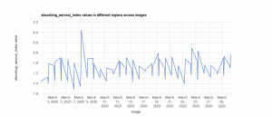
Click on the panel to generate your map
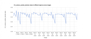
Carbon Monoxide (CO)
Carbon monoxide (CO) is an important atmospheric trace gas for understanding tropospheric chemistry. In certain urban areas, it is a major atmospheric pollutant. Main sources of CO are combustion of fossil fuels, biomass burning, and atmospheric oxidation of methane and other hydrocarbons. Whereas fossil fuel combustion is the main source of CO at northern mid-latitudes, the oxidation of isoprene and biomass burning play an important role in the tropics.
Click on the panel to generate your map
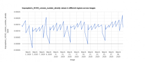
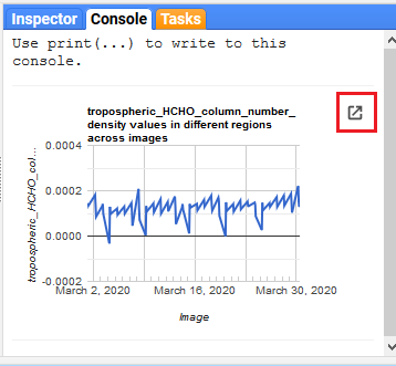
Formaldehyde (HCHO)
Formaldehyde is an intermediate gas in almost all oxidation chains of non-methane volatile organic compounds (NMVOC), leading eventually to CO2. Non-Methane Volatile Organic Compounds (NMVOCs) are, together with NOx, CO and CH4, among the most important precursors of tropospheric O3. The major HCHO source in the remote atmosphere is CH4 oxidation. Over the continents, the oxidation of higher NMVOCs emitted from vegetation, fires, traffic and industrial sources results in important and localized enhancements of the HCHO levels.
Click on the panel to generate your map
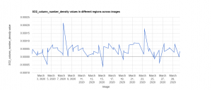
SO2
Sulphur dioxide (SO2) enters the Earth’s atmosphere through both natural and anthropogenic processes. It plays a role in chemistry on a local and global scale and its impact ranges from short-term pollution to effects on climate. Only about 30% of the emitted SO2 comes from natural sources; the majority is of anthropogenic origin. SO2 emissions adversely affect human health and air quality. SO2 has an effect on climate through radiative forcing, via the formation of sulphate aerosols.
Click on the panel to generate your map


 Specify the maximum allowed percent of the clouds content on the pictures by setting the value of the variable cloudFraction.


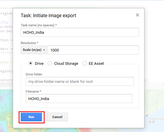
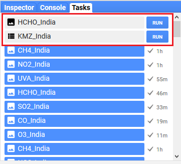 You can choose the highlighted on the yellow colour 'Tasks' tab to download your images (.GeoTiff format) and KMZ file (geometry of the image). To proceed, click Run.